Week 6 Hypothesis Testing I
This week we introduce hypothesis testing for means.
6.1 What we cover this week
- Hypothesis testing for means - one sample
- Hypothesis testing for means - two sample, independent groups
6.2 Readings
Chapter XII in online textbook
Key sections:
- Single Mean
- Difference between 2 means
- Correlated Pairs
- Statistical literacy
6.3 Lab
This lab is due on the Dropbox on MyLearningSpace on Friday March 12th
We are going to explore one of my favourite geospatial technologies for our foray into hypothesis testing, Global Positioning Systems (GPS), which is a specific form of the more general Global Navigation Satellite Systems (GNSS). With the advent of GPS chips in mobile phones, location-aware applications and services are now extremely widely used. The quality of GPS sensors varies considerably and an affect how we use the positioning information we get from them. One particular issue with GPS is that it does not work in doors. If you have even a rough understanding of how GPS works, you will know you have to connect to satellites that receive messages to your receiver, and connecting to multiple satellites allows your exact position on the surface of the earth to be located. If we are inside, we cannot receive signals broadcast from space.
Now this issue can get a little more complex when we are using GPS outdoors in areas where we do not have a clear view of the sky. In particular, GPS signals can reflect off of objects in the path between our receiver and the satellite - a phenoemna known as GPS multipath error as the error is due to the multiple paths the signal takes. More advanced GPS receivers use different techniques to minimize this issue. However, multipath error can still be an issue in urban environments with tall buildings nearby or in forested areas with canopy cover.
In this lab we will compare the GPS signals we received from two receivers - Garmin GPSmap 62s and an Iphone App on an IPhone 8 Plus phone - the EpiCollect 5. Garmin is considered recreational grade while the IPhone app is not a true GNSS receiver. What we want to explore is the difference in reported positioning for these two receivers. To do a proper error analysis of these units, we would really need to compare them to a third independent benchmark, such as a survey marker or a GPS position obtained from a highly accurate positioning system using differential corrections. Lacking that - we will simply compare the positions to each other, to ask; are the positions statistically different.
6.3.1 Examining with Fake Data
We will first create some fake geographic data to examine. One of the great things about working with R is that you can usually find a package to do just about anything you want to do. In this case we want an R function to generate random geographic coordinates. We could for example, use runif which generates random uniform numbers and just set the min and max to -180 and +180 for longitude and -90 and +90 for latitude, but we might want finer control, for example to generate random points within some distance of a known location, or within the bounds of a country or neighbourhood.
#install.packages("randgeo")This line above only ever needs to be run one time - this installs the package on your computer. You need to load the package in order to use it:
library("randgeo")We can see how to work with this package by looking at its documentation website. If you do you will see that the function we want is called rg_position which we can get help for to see its arguments:
?rg_positionwhich you will see takes one argument for the number of points you want and another for a bbox - or a bounding box within which points should be generated. We will use the bbox argument to generate some random points within a specific area. Luckily there is a website that makes this process very easy from which you can copy the bounding box coordinates.
Given that we’re probably all desparate to travel at this point, I am going to go to one of my favorite places I have travelled to, Arugum Bay in Sri Lanka.
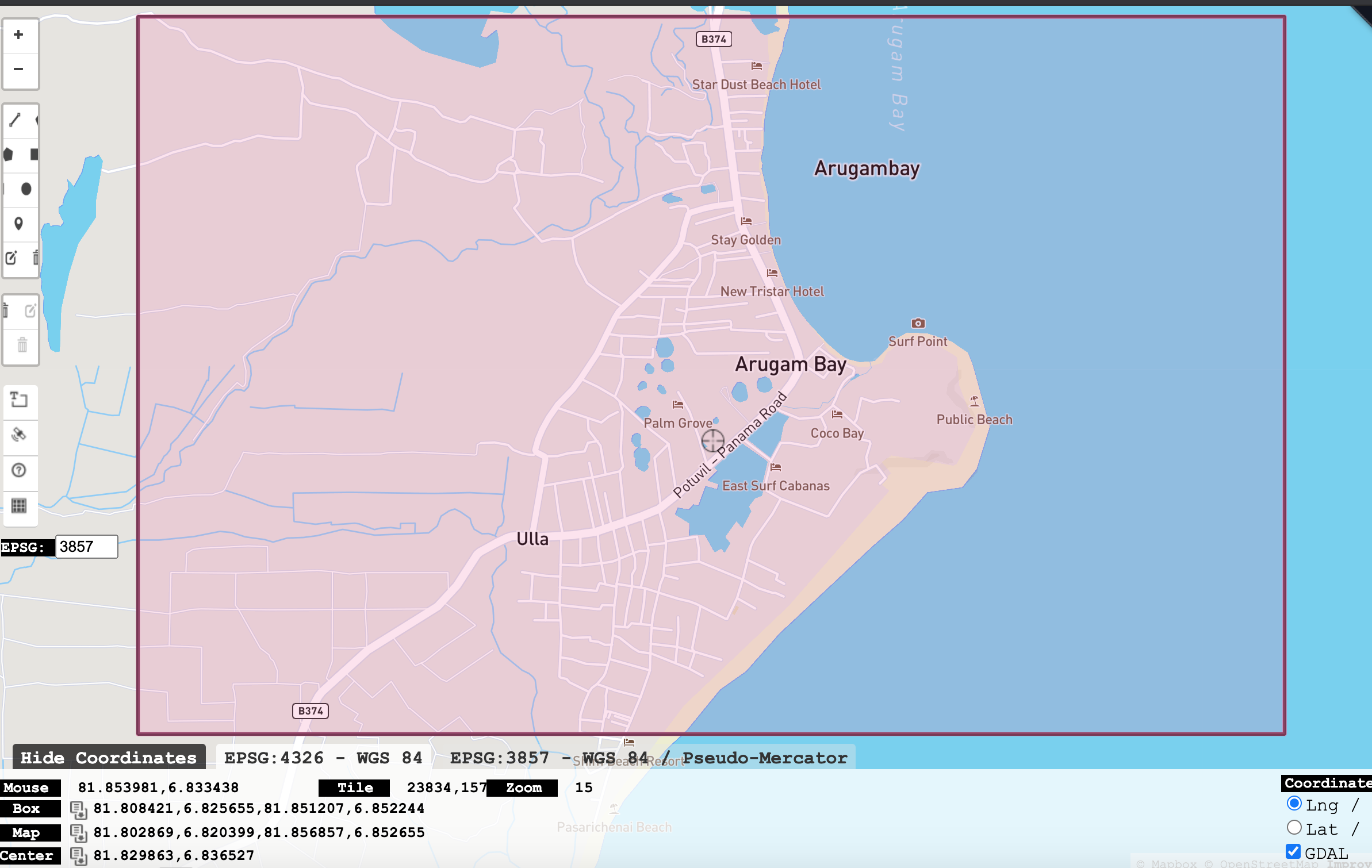
Figure 6.1: Arugam Bay, Sri Lanka.
Feel free to change this somewhere you want to go! For my study area, we can see the bounding box is 81.808421,6.825655,81.851207,6.852244 and this is reported in Longitude, Latitude pairs for the box, and when we look at the rg_position help it tells it that it requires this information as numeric vector of the form west (long), south (lat), east (long), north (lat). Lets try it
rg_position(count = 1, bbox = c(81.808421,6.825655,81.851207,6.852244))## [[1]]
## [1] 81.837524 6.837419Try plugging the result into google maps to see if it lands in the correct location (Google Maps takes latitude/longitude in the search box so you’ll have to switch the order).
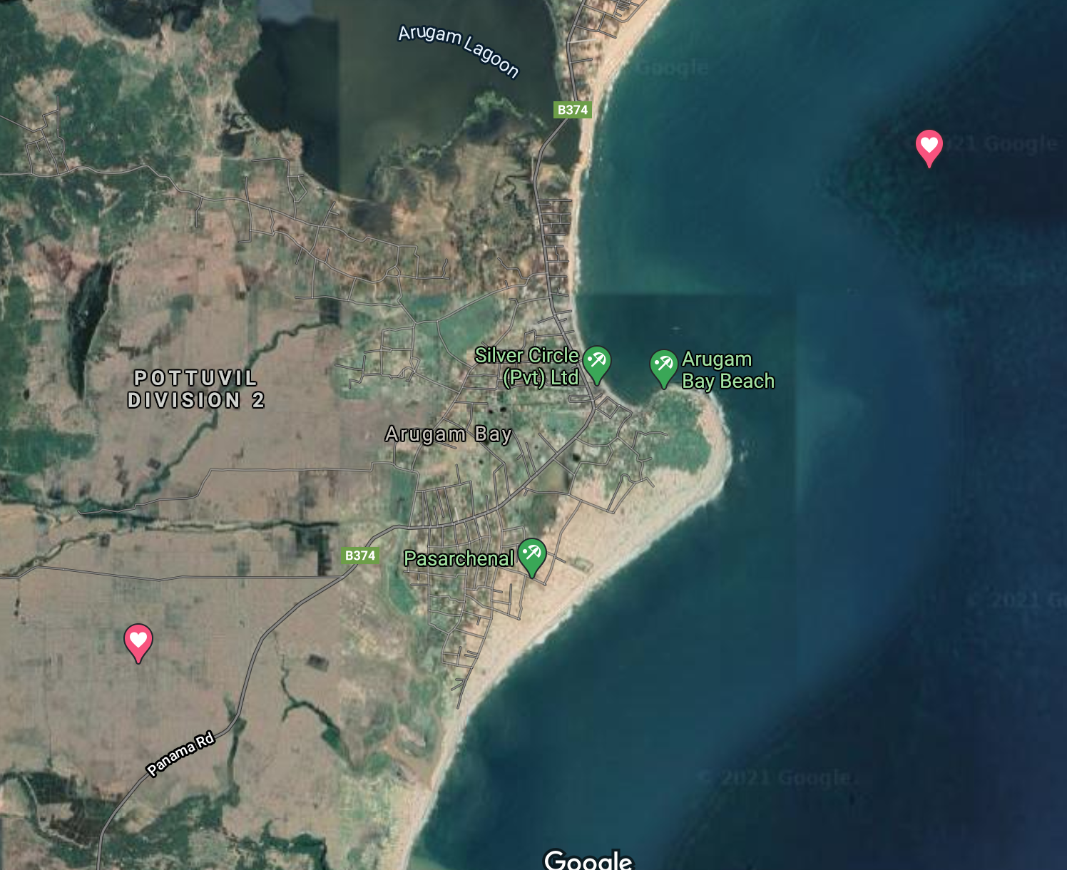
Figure 6.2: Bounding box coordinates plotted on Google Maps
We can get more points by increasing the count argument as follows:
rg_position(count = 5, bbox = c(81.808421,6.825655,81.851207,6.852244))## [[1]]
## [1] 81.820510 6.836621
##
## [[2]]
## [1] 81.812479 6.848507
##
## [[3]]
## [1] 81.839422 6.836808
##
## [[4]]
## [1] 81.820202 6.829456
##
## [[5]]
## [1] 81.841141 6.844486now the rg_position function returns a list of pairs of longitude/latitude pairs. We can convert them to a data frame with a little r magic -
set.seed(123)
df1 <- data.frame(matrix(unlist(rg_position(count = 30, bbox = c(81.808421,6.825655,81.851207,6.852244))), ncol = 2, byrow = TRUE))
df2 <- data.frame(matrix(unlist(rg_position(count = 30, bbox = c(81.808421,6.825655,81.851207,6.852244))), ncol = 2, byrow = TRUE))
so now we have two data frames each with 30 geographic cooridnates in our area of interest.
head(df1)## X1 X2
## 1 81.82073 6.846615
## 2 81.82592 6.849133
## 3 81.84866 6.826866
## 4 81.83102 6.849383
## 5 81.83201 6.837796
## 6 81.84936 6.837709head(df2)## X1 X2
## 1 81.83688 6.828177
## 2 81.82485 6.832950
## 3 81.84328 6.837580
## 4 81.84308 6.847256
## 5 81.84241 6.837350
## 6 81.84070 6.842385Now, back to GPS and hypothesis testing.
We will pretend df1 are coordinates from one GPS and df2 are coordinates from another GPS. Since these were just randomly created we won’t expect the coordinates to be close - but the idea of comparing coordinates will be the same.
6.3.2 One-Sample Hypothesis Testing
First we will test the hypothesis of whether the difference is equal to zero.
\(H_0: \mu = 0\) \(H_A: \mu \ne 0\)
where \(\mu\) is the population mean difference. To start we have to compute our variable analysis. Given that we have a two-dimensional measure of location that we want to summarize with a single vector, we will convert the geographic coordinates to distance using pythagorous theorum which in r is just implementing \(d = \sqrt{(x_1-x_2)^2 + (y_1-y_2)^2}\) as follows
d <- sqrt((df1$X1 - df2$X1)^2 + (df1$X2 - df2$X2)^2)so now we are testing \(H_0: \mu = 0\) on the sample mean difference in d.
The function for doing a t-test in r is t.test.
t.test(d, mu=0)##
## One Sample t-test
##
## data: d
## t = 11.851, df = 29, p-value = 1.227e-12
## alternative hypothesis: true mean is not equal to 0
## 95 percent confidence interval:
## 0.01592541 0.02256879
## sample estimates:
## mean of x
## 0.0192471As per lecture slides the way we calculate a t-statistic for our vector d is:
\(t = \frac{\bar{x} - \mu}{\sigma_{\bar{x}}}\)
where \(\sigma_{\bar{x}}\) is \(\frac{s}{\sqrt{n}}\) which we can hand-calculcate in r as:
mean(d) / (sd(d)/sqrt(30))## [1] 11.85081which can see matches the output of the t.test function for the value of the t. We can evaluate probability as well:
pt(q = 11.85081, df = 29)## [1] 1now what would happen if we actually wanted to test
\(H_0: \mu = 0.02\)
\(H_A: \mu \ne 0.02\)
the above would change to
(mean(d) - 0.02) / (sd(d)/sqrt(30))## [1] -0.4635751Can you see how our conclusion would change and what this would mean? How would result from pt change?
6.3.3 Two-Sample Hypothesis Testing
Lets suppose that the first 14 of our data points were collected on a day with overcast weather, and the remaining 16 points were collected on a clear day. We might want to examine whether there was a statistical difference between the two days. This would be comparing two groups; and we would need a two-sample hypothesis test to evaluate:
\(H_0: \mu_1 = \mu_2\)
\(H_A: \mu_1 \ne \mu_2\)
which is to say, there is not a difference (ie the two means are equal) or there is (ie the two means are not equal). First we need to separate out the two groups. We can do this by subsetting into two new vectors as follows:
day1 <- d[1:14]
day2 <- d[15:30]
then we test using t.test again:
t.test(day1, day2)##
## Welch Two Sample t-test
##
## data: day1 and day2
## t = -0.94932, df = 24.489, p-value = 0.3517
## alternative hypothesis: true difference in means is not equal to 0
## 95 percent confidence interval:
## -0.009495550 0.003508026
## sample estimates:
## mean of x mean of y
## 0.01765043 0.02064419This result shows there is no statistical difference between the values in d between day 1 and day 2 because the p-value associated with the null hypothesis is p=0.3517 which is far greater than any of the nominal significance levels we use in hypothesis testing. Note that the df is different here and no longer n-1 as in the case with single sample hypothesis testing.
6.3.4 GPS Dataset
I collected some GPS data using two method described above, the EpiCollect App for IPhone and a Garmin GPS Receiver. Below is a video showing some details of the data collection process, as well as a lengthy illustration of how we bring the field data into R. This may only be of interest to some students.
The data can be accessed as follows:
df <- read.csv("https://www.dropbox.com/s/f7xcibye2epgqgy/dfprocessed.csv?dl=1")
open_dis <- df$dis[which(df$loctype=="Open")]
forest_dis <- df$dis[which(df$loctype=="Forest")]
mean(open_dis)
## [1] 24.51924mean(forest_dis)## [1] 30.334746.3.5 Lab Assignment
Generate random points for a study area of interest to you (as in the example above). Conduct a hypotheses test that the mean difference is a) equal to zero then b) greater than 0.02. For each use the
t.testfunction as well as the hand-calculated method shown in the instructions above to confirm your answer. In your answer include your hypothesis statements, p-value, and a sentence interepting your results from each hypothesis test. Include a screenshot showing your bounding box coordinates plotted on Google Maps (out of 5)For the GPS data, is the mean difference significantly different from zero (\(\alpha = 0.05\))? Use the
t.testfunction as well as the hand-calculated method shown in the instructions above to confirm your answer. In your answer include your hypothesis statements, p-value, and a sentence interepting your results from each hypothesis test. (out of 5)For the GPS data, was the difference between the two receivers statistically different between locations under forest canopy vs .open sky? Was there more or less difference when under forest canopy? Conduct both one tailed and two tailed hypothesis tests. For this question you can just use the
t.testfunction. In your answer include your hypothesis statements, p-value, and a sentence interepting your results from each hypothesis test. (out of 5)For the GPS data, test whether the distance between the two receivers were statistically lower when accuracy was low (<=12, vs high >12). For this question you can just use the
t.testfunction. In your answer include your hypothesis statements, p-value, and a sentence interepting your results from each hypothesis test. (out of 5)